Dictionary Learning with Sparse AutoEncoders
Taking Features Out of Superposition
Mechanistic Interpretability
Given a task that we don’t know how to solve directly in code (e.g. recognising a cat or writing a unique sonnet), we often write programs which in turn, (via SGD), write second-order programs. These second-order programs (i.e. neural network weights) can solve the task, given lots of data.
Suppose we have some neural network weights which describe how to do a task. We might want to know how the network solved the task. This is useful either to (1) understand the algorithm better for ourselves or (2) check if the algorithm follows some guidelines we might like e.g. not being deceptive, not invoking harmful bias etc.
The field of Mechanistic Interpretability aims to do just that - given a neural
network1, return a correct, parsimonious, faithful and
human-understandable explanation of the inner workings of the network when
solving a given task. This is analogous to the problem of
reverse engineering software from machine code
or the problem of a
neuroscientist trying to understand the human brain.
💭 The Dream
How are we to translate giant inscrutable matrices into neat explanations and high-level stories?
In order for a neural network to make some prediction, it uses internal neuron activations as “variables”. The neuron activations build up high-level, semantically rich concepts in later layers using lower-level concepts in earlier layers.
A dream of Mechanistic Interpretability would be this:
Suppose we had some idea that each neuron corresponded to a single feature. For example, we could point to one neuron and say “if that neuron activates (or “fires”) then the network is thinking about cats!”. Then we point to another and say “the network is thinking about the colour blue”. Now we could give a neural network some inputs, look at which internal neurons activate (or “fire”) and use this to piece together a story about how the network came up with its eventual prediction. This story would involve knowing the concepts (“features”) the network was “thinking” about together with the weights (“circuits”) which connect them.
This would be great! Unfortunately, there are a couple of problems here…
👻 The Nightmare
Firstly, neural networks are freaking huge. There can be literally billions of weights and activations relevant for processing a single sentence in a language model. So with the naive approach above, it would be an incredibly difficult practical undertaking to actually tell a good story about the network’s internal workings2.
But, secondly, and more importantly, when we look at the neurons of a neural network we don’t see the concepts that it sees. We see a huge mess of concepts all enmeshed together because it’s more efficient for the network to process information in this way. Neurons that don’t activate on a single concept but instead activate on many distinct concepts are known as polysemantic neurons. It turns out that basically all neurons are highly polysemantic3.
In essence, neural networks have lots of features, which are the
fundamental units (“variables”) in neural networks. We might think of features
as directions in neuron space corresponding to the concepts. And neurons are
linear combinations of these features in a way that makes sense to the network
but looks very entangled to us - we can’t just read off the features from
looking at the activations.
Sparse Dictionary Learning As A Solution
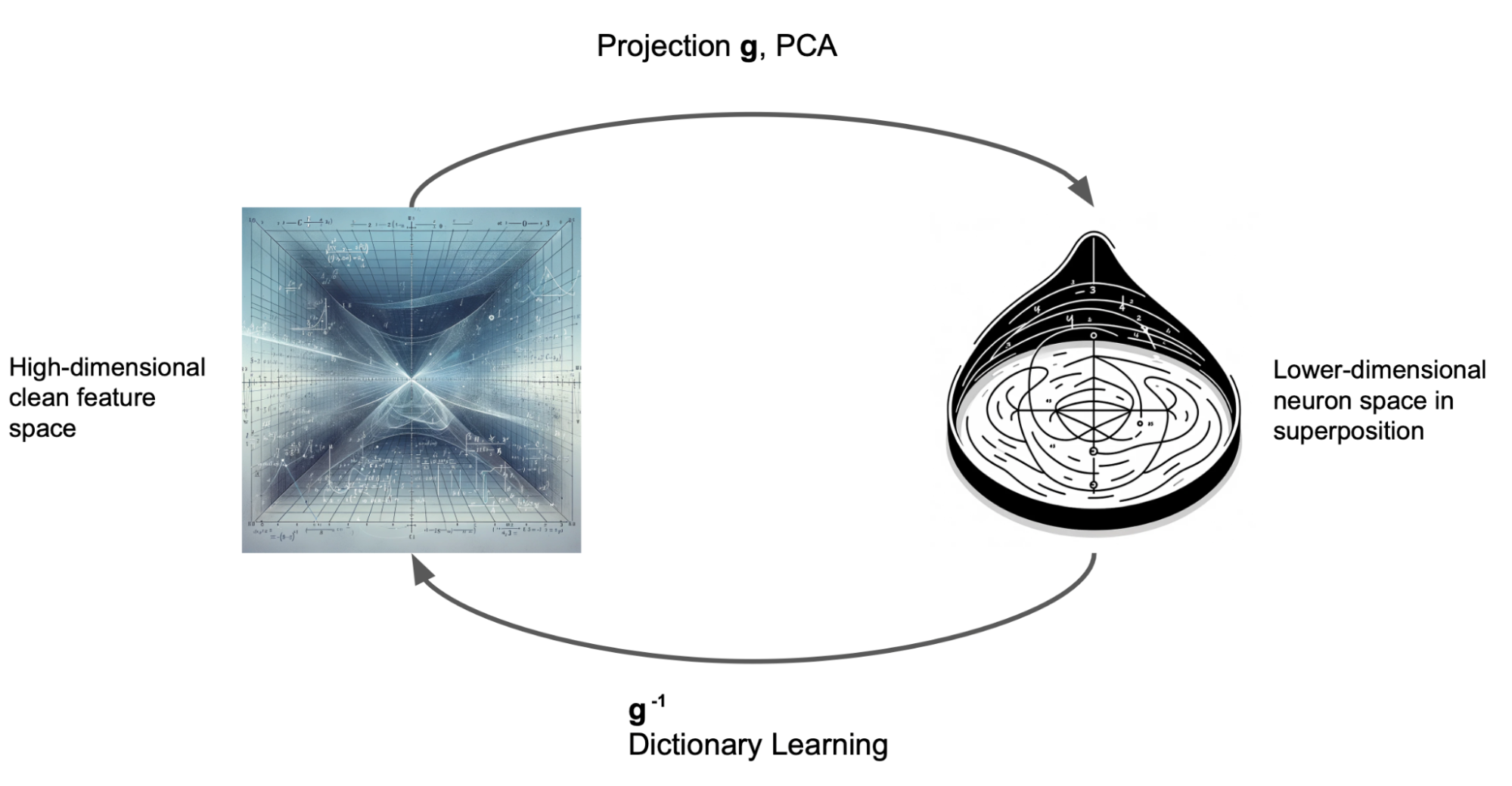
So we’re given a network and we know that all the neurons are linear combinations of the underlying features but we don’t know what the features are. That is, we hypothesise that there is some linear map g from the feature space to neuron space. Generally, feature space is much bigger than neuron space. That is to say, there are more useful concepts in language than the number of neurons that a network has. So our map g is a very rectangular matrix: it takes in a large vector and outputs a smaller one with the number of neurons as the number of dimensions.
We want to recover the features. To do this we could try to find a linear function which can map from neuron space → feature space and acts as the inverse of g. We go to our Linear Algebra textbook (or ask ChatGPT) how to invert a long rectangular matrix and it says… oh wait, yeah this actually isn’t possible4. A general linear map from feature space → neuron space loses information and so cannot be inverted - we can’t recover the features given only the neurons.
This seems bad but let’s soldier on. Instead of giving up, we instead ask, “okay well we can’t invert a general linear map g but what constraints could we put on g such that it might be invertible?” As it turns out, if most of the numbers in the matrix corresponding to g are 0 (that is if g is sufficiently sparse) then we can invert g.5
Q: Hold on, is this reasonable? Why might we expect g to be (approximately) sparse?
In predicting the next token there will be some relevant features of the previous tokens which are useful. If the neural network has tens of thousands of features per layer (or perhaps even more), then we would expect some of them to be useful for each prediction. But if the prediction function uses all of the features it would be super complex; most features should be irrelevant for each prediction.
As an example consider if you’re deciding if a picture of an animal is a dog - you might ask “does it have 4 legs?” - 4 legged-ness is a useful feature. The texture of its fur is also relevant. The question “would a rider sit within or on top” is probably not relevant, though it might be relevant in other situations for example distinguishing a motorbike from a car. In this way, not all of the features are needed at once6.
To recap, so far we’ve said:
- Language models use features in order to predict the next token.
- There are potentially a lot more features than there are neurons.
- If the linear map g: features → neurons was sparse then we might be able to find an inverse.
- Sparse maps are relatively good approximations to the real linear map g.
Sparse Dictionary Learning is a method which exploits these facts to numerically find the inverse of g. Intuitively what we have is a lookup table (or a “dictionary”) which tells us how much of each feature goes into each neuron. And if these features look monosemantic and human-understandable then we’re getting very close to the dream of Mechanistic Interpretability outlined above. We could run a model, read off the features it used for the prediction and build a story of how it works!
Dictionary Learning Set-up
We’ll focus here on Anthropic’s set-up.
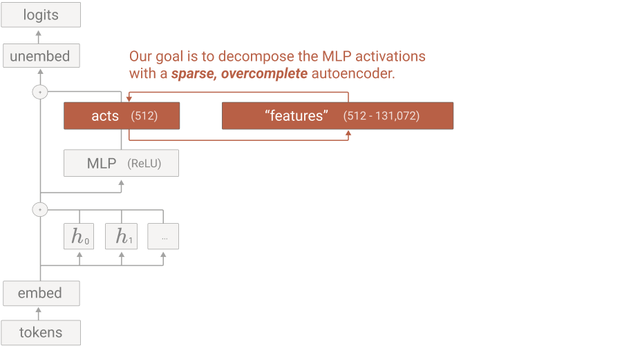
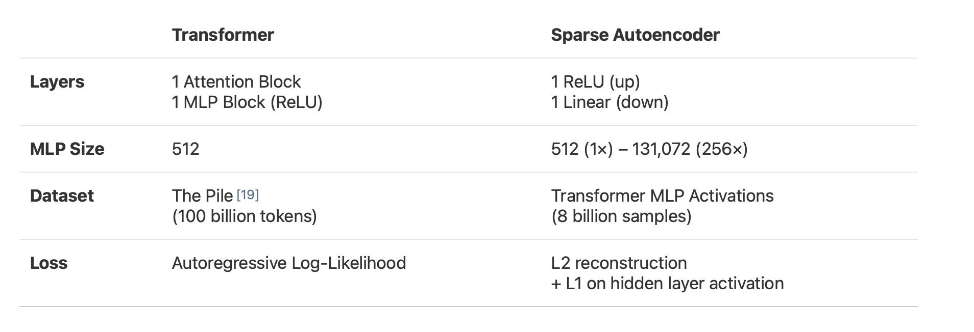
We start with a small 1-Layer transformer which has an embedding dimension of 128. Here the MLP hidden dimension is 512.7 The MLP contains:
- An up_projection to MLP neuron space (512d),
- A ReLU activation which produces activations and then
- A down_projection back to embedding space (128d)
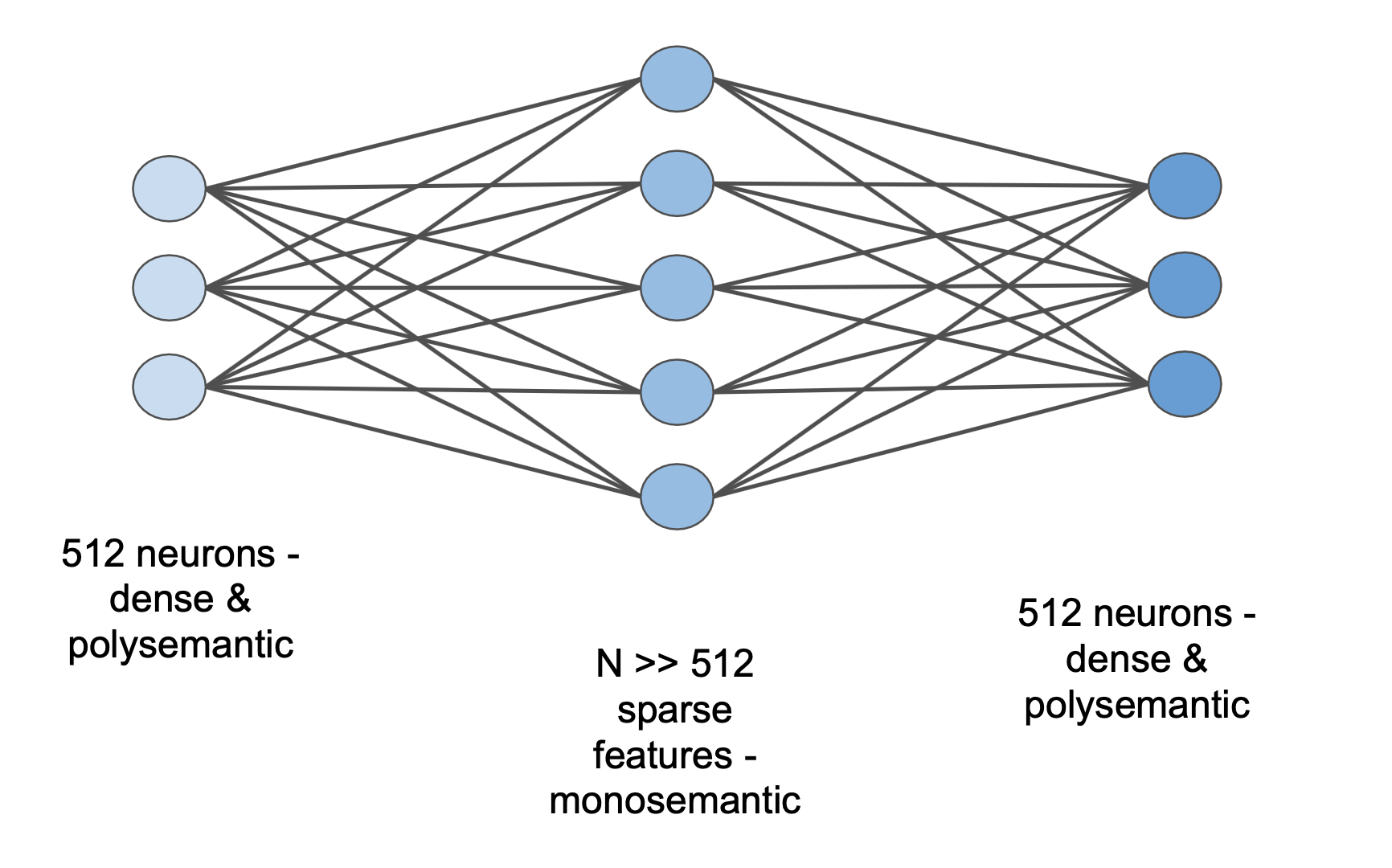
We capture the MLP neuron activations and send those through our sparse autoencoder which has N dimensions for some N ≥ 512.
An AutoEncoder is a model which tries to reconstruct some data after putting it through a bottleneck. In traditional autoencoders, the bottleneck might be mapping to a smaller dimensional space or including noise that the representation should be robust to. AutoEncoders aim to recreate the original data as closely as possible despite the bottleneck. To achieve the reconstruction, we use a reconstruction loss which penalises outputs by how much they differ from the MLP activations (the inputs to the AutoEncoder).
In the Sparse AutoEncoder setting, our “bottleneck” is actually a higher
dimensional space than neuron space (N ≥ 512), but the constraint is that the
autoencoder features are sparse. That is, for any given set of MLP neuron
activations, only a small fraction of the features should be activated.
In order to make the hidden feature activations sparse, we add an L1 loss over the feature activations to the reconstruction loss for the AutoEncoder’s loss function. Since the L1 loss gives the absolute value of the vector, minimising L1 loss pushes as many as possible of the feature activations towards zero (whilst still being able to reconstruct the MLP neurons to get low reconstruction loss).
To recap:
- The input of the AutoEncoder is the MLP activations.
The goal is for the output of the AutoEncoder to be as close to the input as possible - the reconstruction loss penalises outputs by how much they differ from the MLP activation inputs.
- The bottleneck is the sparsity in the hidden layer which is induced by pressure from the L1 loss to minimise feature activations.
In summary, the set-up Anthropic uses is:
Anthropic’s Results
The most surprising thing about this approach is that it works so well. Like really well.
There are, broadly, two ways to think about features:
- Features as Results - the feature activates when it sees particular inputs. Looking at features can help us to understand the inputs to the model.
- Features as Actions - ultimately features activating leads to differences in the output logits. Features can be seen as up-weighting or down-weighting certain output tokens. In some sense, this is the more fundamental part. If we ask “what is a feature for?” then the answer is “to help the model in predicting the next token.”
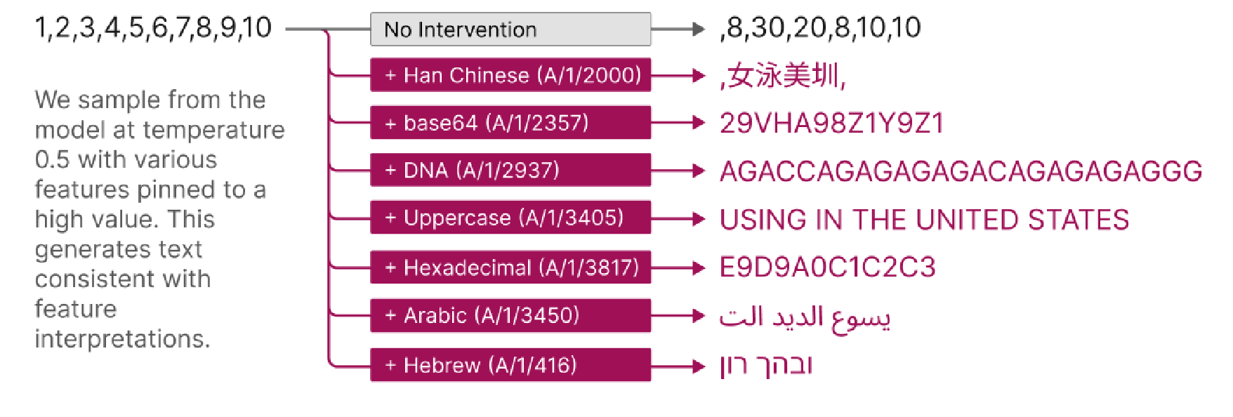
Anthropic find many features which activate strongly in a specific context (say
Arabic script or DNA base pairs) and also (mostly) only activate when that
context is present. In other words, the features have high
precision and recall. This
suggests that these are ~monosemantic features! In terms of
Features as Results, this captures what we would hope for - the features that
appear are mostly human-understandable.
The authors also find that once a feature is activated, the result is an
increase in plausible next tokens given the input. In particular, to demonstrate
this counterfactually, we can add a large amount of a given feature to the
neuron activations. Theoretically, this should “steer” the model to thinking
that context was present in the input, even if it wasn’t. This is a great test
for Features as Actions.
Additionally, if we fully replace the MLP activations with the output of our
autoencoder8, we get a model which explicitly uses our feature dictionary
instead of the learned MLP neurons. Here the resulting “dictionary model” is
able to get 95% of the performance of the regular model. The dictionary model
achieves this despite, in the case of large autoencoders, the features being
extremely sparse. This performance is a great sign for Features as Actions; it
suggests that the sparse features capture most of the information that the model
is using for its prediction task! This also validates that our assumption that
features are approximately sparse seems to be a fairly good assumption9.
Other Phenomena
They also note some other smaller results:
- As the number of features in the autoencoder increases, we capture more of the true performance of the model. This correlation suggests that models are probably implementing up to 100x or more features than they have neurons 🤯
- The features are generally understandable by both humans and by other Machine Learning models. To show this they ask Claude to do some interpretation too.
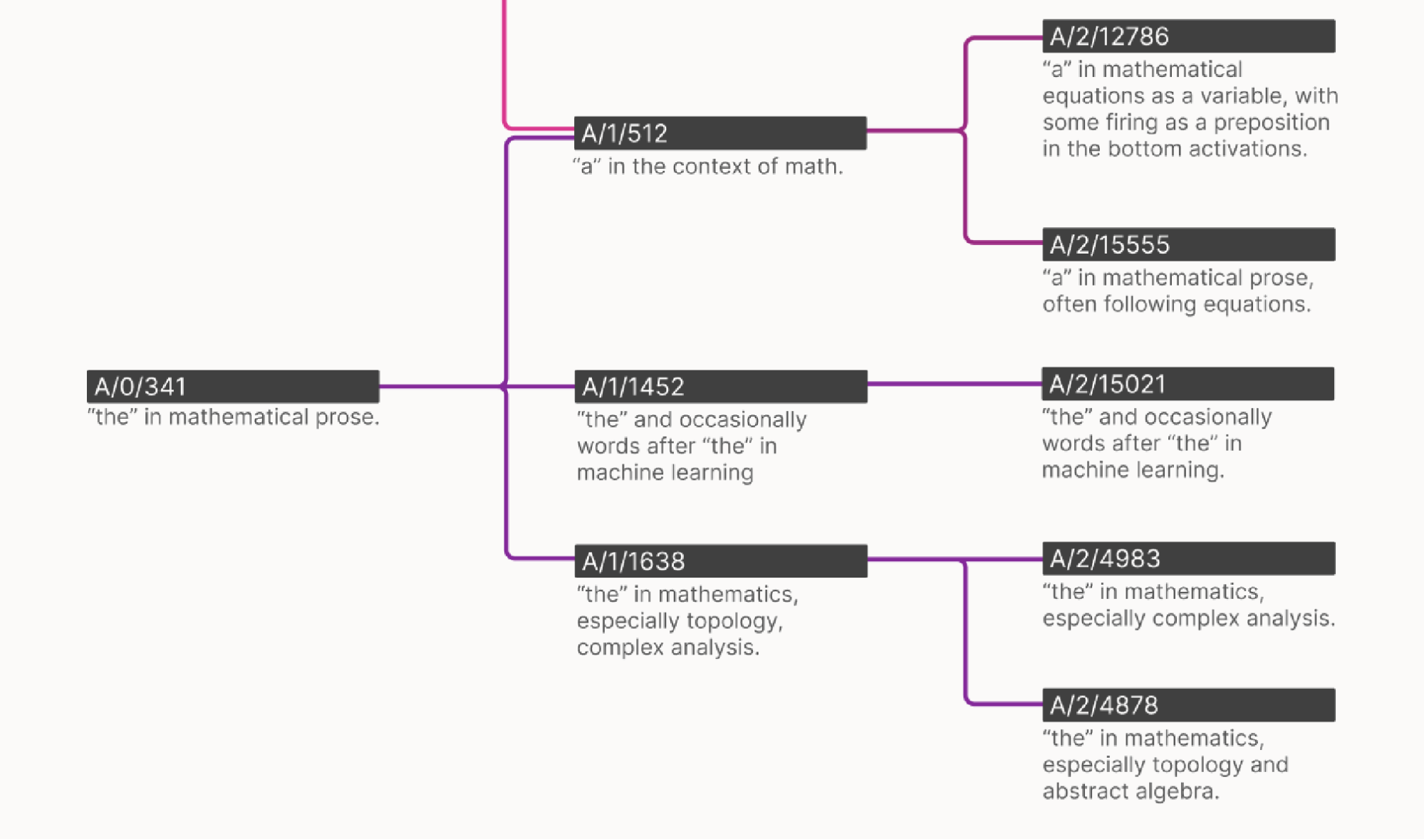
- As the number of features increases, the features themselves “split”. That is even though a feature is monosemantic - it activates on a single concept - there may be levels to concepts. For example, small autoencoders might have a (monosemantic) feature for the concept “dog”. But larger autoencoders have features for corgis and poodles and large dogs etc. which break down the concept of dog into smaller chunks. Scale helps with refining concepts.
What’s Next?
Have All The Problems in Mechanistic Interpretability Been Solved?
Certainly not. Although this approach is a breakthrough in approaching features and converting regular networks into less polysemantic ones, some problems remain:
📈 Scaling Sparse Autoencoders
Large models are still, well … large. Dictionary learning mitigates the problem since we don’t have to deal with polysemantic neurons anymore. But there’s still a lot that could happen between doing this on a small 1-Layer model and a large model. In particular, since there are many more features than neurons, Sparse AutoEncoders for large models could be absolutely gigantic and may take as much compute to train as the model’s pre-training. We will very likely need ways to improve the efficiency of Sparse AutoEncoder training.
🤝 Compositionality and Interaction Effects
In Machine Learning, as in Physics, More Is Different. That is, there may be qualitatively different behaviours for large models as compared to smaller ones. One clear way this could occur is when features are composed of many sub-features across different layers and form complex interactions. This is an open problem to be explored.
🌐 Universality
The Universality Hypothesis from Chris Olah states that sufficiently neural networks with different architectures and trained on different data will learn the same high-level features and concepts.
The authors show that when two models are trained with the same architecture but different random initialisations, they learn similar features. This is certainly a step towards universality but doesn’t show the whole thesis. A strong form of Universality would suggest that there are some high-level “natural” features/concepts which lots of different architectures for predictors (silicon and human brains) all converge on. We’re quite a way from showing this in the general case.
📐 Interpretability Metrics
Though there are some proxy measures for interpretability, currently the best metric that we have is for a human to check and say “yes I can interpret this feature” or “no I can’t”. This seems hard to operationalise at scale as a concrete metric.
To bridge this gap large models such as GPT-4 and Claude can also help with the interpretability. In a process known as AutoInterpret, LLMs are given a prompt and how much each feature activates. They then attempt to interpret the feature. This works kinda okay at the moment but it feels like there should be a cleaner, more principled approach.
☸︎ Steering
The authors show that by adding more of a given feature vector in activation space, you can influence a model’s behaviour. When, whether, and how steering works reliably and efficiently are questions that could all be useful. We might wish to steer models as a surgical needle to balance out the more coarse tool that is RLHF. In the future, this may also be useful to reduce harmful behaviour in increasingly powerful models.
🔳 Modularity
As mentioned above, there would be an embarrassingly large number of features for a model like GPT-4 and so it looks like it will be difficult to create succinct compelling stories which involve so many moving parts. In some sense, this is the lowest level of interpretability. It’s analogous to trying to understand a very complex computer program by looking through it character by character, if the words were all jumbled up.
What we would like is some slightly higher level concepts composed of multiple features with which we can use to think. Splitting up the network into macro-modules rather than the micro-level features seems like a promising path forward.
Conclusion
Anthropic are very positive about this approach and finish their blog post with the line:
For the first time, we feel that the next primary obstacle to interpreting large language models is engineering rather than science.
There is some truth to how exciting this development is. We might ask whether the work ahead is purely scaling up. As we outlined in the problems for future work above, I do believe there are still some Science of Deep Learning problems which Mechanistic Interpretability can sink its teeth into. Only now, we also have a new tool which is incredibly powerful to help us along the way.
In light of the other problems that still remain to be solved, we might add the final sentences of Turing’s 1950 paper, as an addendum:
We can only see a short distance ahead, but we can see plenty there that needs to be done.
Thanks to Derik and Joe for comments on a draft of this post.
-
With both its weights and its activations on a series of input examples say ↩
-
Of course, if it’s just a practical undertaking perhaps we would grit our teeth and try to do this - it appears we at least have the tools to give it a shot, even if it’s painfully slow. We have completed huge practical undertakings before as a scientific community e.g. deciphering the human genome or getting man to the moon. As we will see there is another concern as well. ↩
-
One theory of exactly how that might come about is found in the Superposition Hypothesis. ↩
-
Thanks to Robert Huben for this useful framing ↩
-
The proof of this and the convergence properties are analogous to how you can use fewer data points for linear regression if you know that the linear map you’re trying to find is sparse e.g. with Lasso methods for sparse linear regression. For this to work precisely, we add a bias and a ReLU non-linearity. ↩
-
This is similar to the intuition of the MoEification paper - MLPs naturally learn some sparse/modular structure, which we might hope to exploit. ↩
-
With the convention from GPT-2 that MLP_dim = 4 * embedding_dim ↩
-
which, we recall, is trying to reconstruct the MLP activations through the sparse bottleneck ↩
-
To the extent that we don’t get 100% of the performance, there are a few hypotheses. Firstly, we might not have the optimal autoencoder architecture yet or the autoencoder might not be fully trained enough to saturation. Secondly, altering the l1loss coefficient hyperparameter adjusts how sparse we want to make our features and there may be some tuning to do there. Thirdly, the network might just not _fully sparse, this seems likely - there are some early results showing that as the size of the model increases (from the toy model we have to a large frontier model), we might expect more sparsity - which suggests that Dictionary Learning may get better with scale. The later Cookbook Features paper also suggests this. ↩
If you'd like to cite this article, please use:
  @misc{kayonrinde2023dictionary-learning,
    author = "Kola Ayonrinde",
    title = "Dictionary Learning with Sparse AutoEncoders",
    year = 2023,
    howpublished = "Blog post",
    url = "http://www.kolaayonrinde.com/2023/11/03/dictionary-learning.html"
  }