DeepSpeed’s Bag of Tricks for Speed & Scale

An Introduction to DeepSpeed for Training

In the literature and the public conversation around Natural Language Processing, lots has been made of the results of scaling up data, compute and model size. For example we have the original and updated transformer scaling laws.

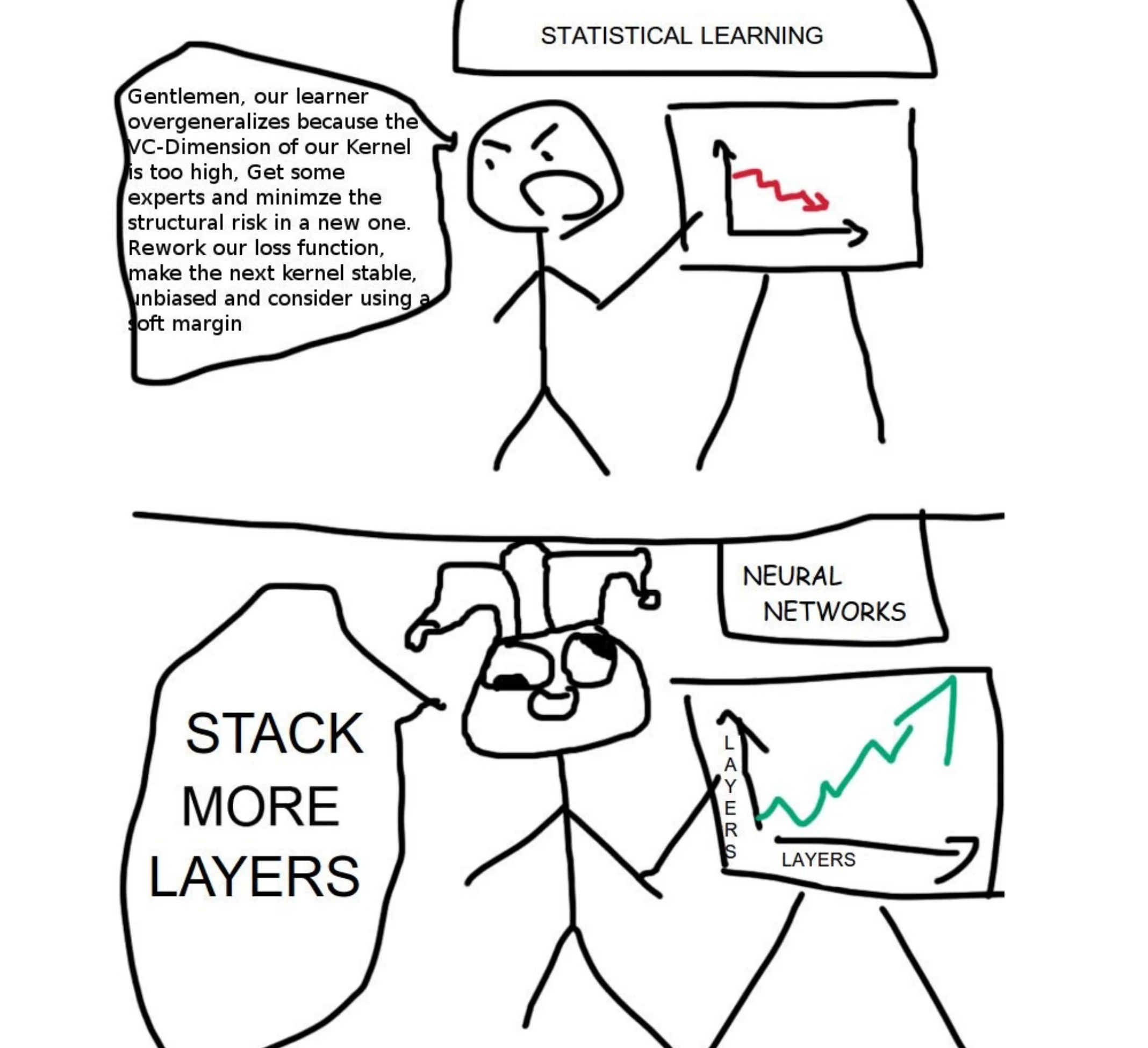
One sometimes overlooked point is the vital role of engineering breakthroughs in enabling large models to be trained and served on current hardware.

This post is about the engineering tricks that bring the research to life.

Note: This post assumes some basic familiarity with PyTorch/Tensorflow and transformers. If you’ve never used these before check out the PyTorch docs and the Illustrated Transformer. Some background on backpropagation works will also be useful - check out this video if you want a refresher!

Table of Contents

0. Introduction
- 0.1 DeepSpeed's Three Innovation Pillars
- 0.2 Problems Training Large Models
1. Partial Solutions
2. DeepSpeed Deep Dive: Key Ideas
3. In Pictures
4. In Code
5. Using DeepSpeed

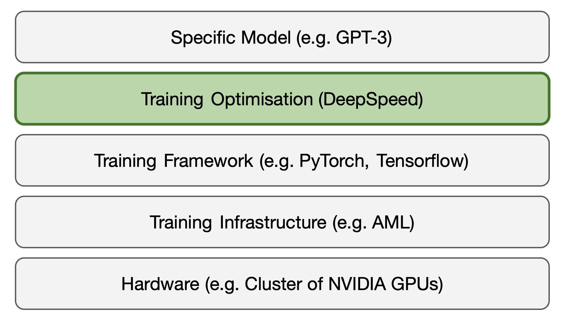
0.1 DeepSpeed’s Three Innovation Pillars

DeepSpeed has four main use cases: enabling large training runs, decreasing inference latency, model compression and enabling ML science.

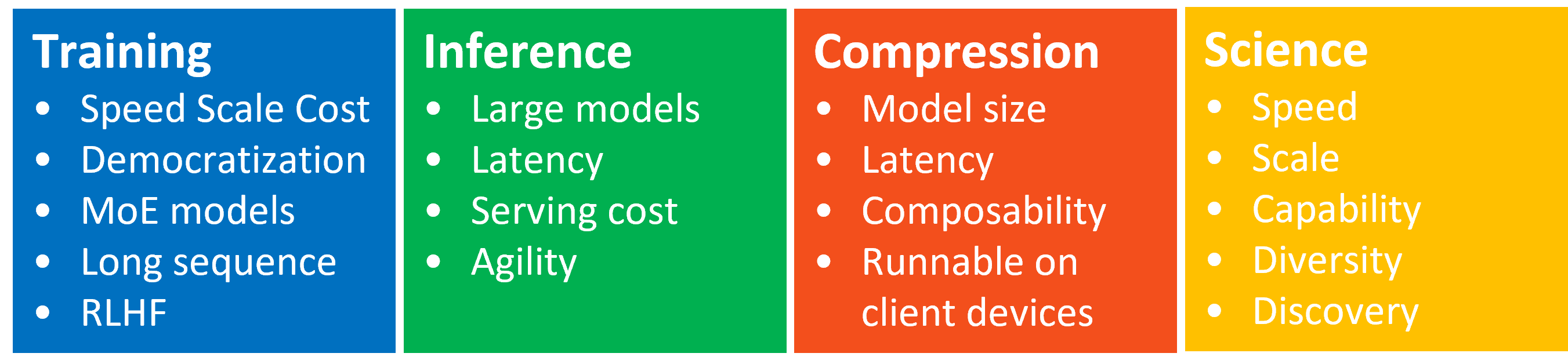
This post covers training optimizations.

0.2 Problems Training Large Models

Training large models (e.g. LLMs) on huge datasets can be can be prohibitively slow, expensive, or even impossible with available hardware.

In particular, very large models generally do not fit into the memory of a single GPU/TPU node. Compared to CPUs, GPUs are generally higher throughput but lower memory capacity. (A typical GPU may have 32GB memory versus 1TB+ for CPUs).

Our aims are:

To train models too large for a single device
Efficiently distribute computation across devices
Fully utilize all devices as much as possible
Minimize communication bottlenecks between devices

DeepSpeed reduces compute and time to train by >100x for large models.

If you just want to see how to implement DeepSpeed in your code, see the Using DeepSpeed section below.

1. Partial Solutions

1.1 Naive Data Parallelism

Without any data parallelism, we get this sorry sight:

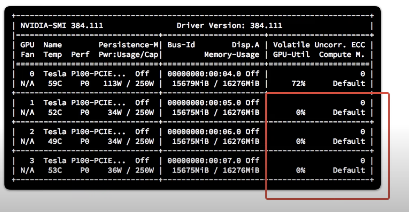
We’ve spent a lot of money on GPU cores for them all to sit there idle apart from one! Unless you’re single-handedly trying to prop up the NVIDIA share price, this is a terrible idea!

One thing that we might try is splitting up the data, parallelising across devices. Here we copy the entire model onto each worker, each of which process different subsets of the training dataset.

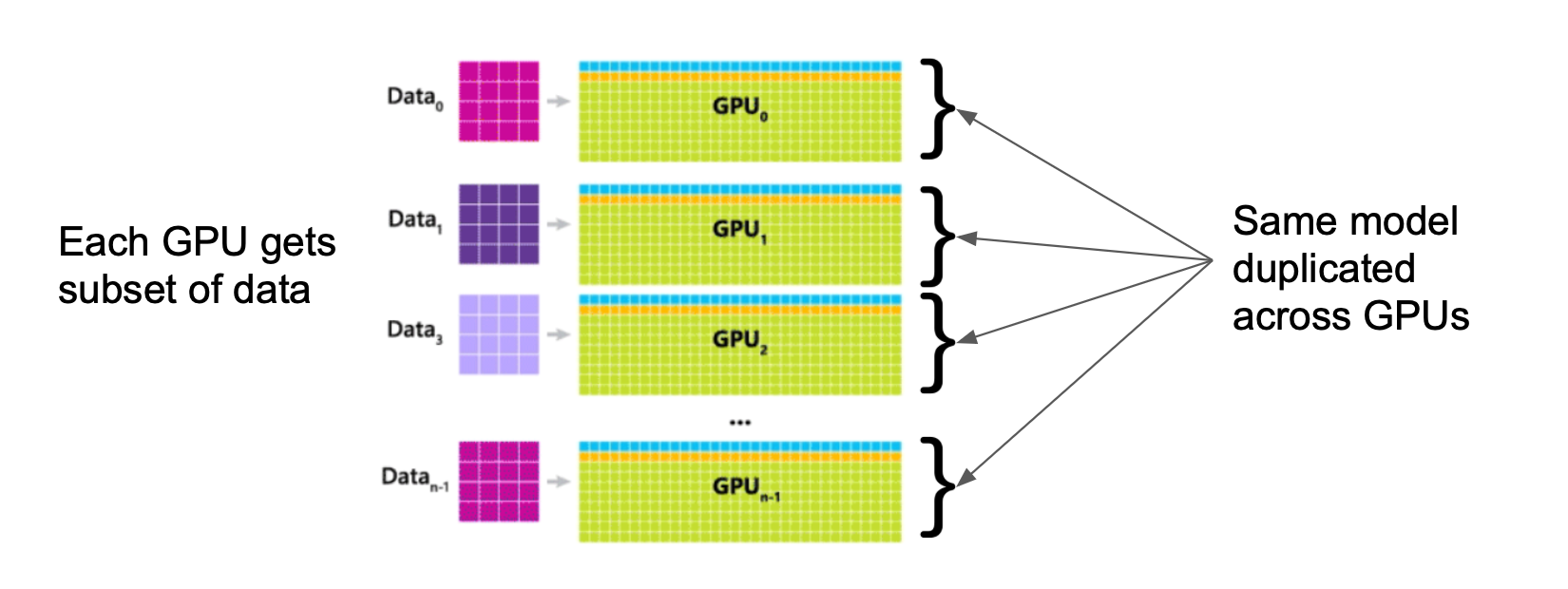
Each device compute its own gradients and then we average out the gradients across all the nodes to update our parameters with all_reduce. This approach is pretty straightforward to implement and works for any model type.

We’ve turned more GPUs into more speed - great!

In addition we also increase effective batch size, reducing costly parameter updates. Since with larger batch sizes there is more signal in each gradient update, this also improves convergence (up to a point).

What's The Catch — I thought you'd never ask

Unfortunately the memory bottleneck still remains. For Data Parallelism to work, the entire model has to fit on every device, which just isn’t going to happen for large models.

1.2 Naive Model Parallelism

Another thing we could try is splitting up the computation of the model itself, putting different layers (transformer blocks) on different devices. With this model parallelism approach we aren’t limited by the size of a memory of a single GPU, but instead by all the GPUs that we have.

However two problems remain. Firstly how to split up a model efficiently is very dependant on the specific model architecture (for example the number of layers and attention heads). And secondly communicating between nodes now bottlenecks training.

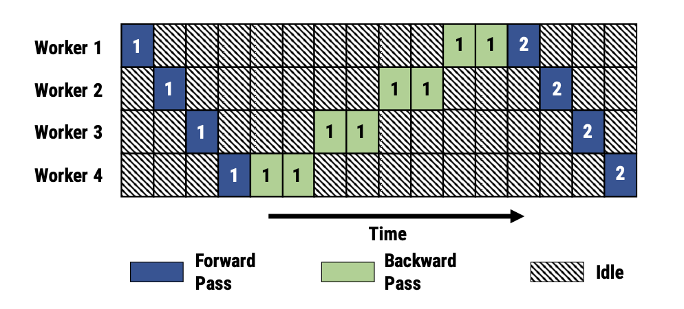
Model parallelisation — One batch moving through the parallelised model. In model parallelisation, one forward and backward pass requires all the devices, most of which are idle at any one time

Since each layer requires the input to the previous layer in each pass, workers spend most of their time waiting. What a waste of GPU time! Here it looks like the model takes the same amount of time as if we had a GPU to fit it on but it’s even worse. The communication overhead of getting data between nodes makes it even slower than a single GPU.

Can we do better than this?

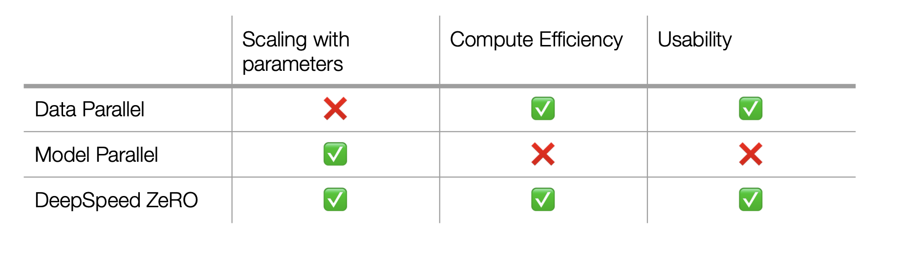
1.3 A Better Way: DeepSpeed

Data Parallelism gave speedups but couldn’t handle models too large for a single machine. Model Parallelism allowed us to train large models but it’s slow.

We really want a marriage of the ideas of both data and model parallelism - speed and scale together.

We don’t always get what we want, but in this case we do. With DeepSpeed, Microsoft packaged up a bag of tricks to allow ML engineers to train larger models more efficiently. All in, DeepSpeed enables >100x lower training time and cost with minimal code changes - just 4 changed lines of PyTorch code. Let’s walk through how.

DP vs MP — Data Parallelisation vs Model Parallelism

2. DeepSpeed Deep Dive: Key Ideas

~~One~~ Seven Weird Tricks to Train Large Models:

Mixed precision training
Delaying Weight Updates
Storing the optimiser states without redundancy (ZeRO stage 1)
Storing gradients and parameters without redundancy (ZeRO stages 2 & 3)
Tensor Slicing
Gradient Checkpointing
Quality of Life Improvements and Profiling

2.0 Mixed Precision Training

Ordinarily mathematical operations are performed with 32 bit floats (fp32). Using half precision (fp16) vs full precision (fp32) halves memory and speeds up computation.

We forward/backward pass in fp16 for speed, keeping copies of fp32 optimizer states (momentum, first order gradient etc.) for accuracy. The high precision fp32 maintains the high dynamic range so that we can still represent very slight updates.

2.1 Delaying Weight Updates

A simple training loop might contain something like:

for i, batch in enumerate(train_loader):

    for j, minibatch in enumerate(batch):

        loss = model(minibatch)
        local_gradients = gradients(loss / batch_size)
        average_gradients = distributed.all_reduce(local_gradients) # reduce INSIDE inner loop

    optimizer.step(average_gradients)

Note here that within every loop we’re calculating not only the local gradients but also synchronizing gradients which requires communicating with all the other nodes.

Delaying synchronization improves throughput e.g:

for i, batch in enumerate(train_loader):

    for j, minibatch in enumerate(batch):

        loss = model(minibatch)
        local_gradients = gradients(loss / batch_size)

    average_gradients = distributed.all_reduce(local_gradients) # reduce OUTSIDE inner loop
    optimizer.step(average_gradients)

2.2 Storing Optimiser States Without Redundancy (ZeRO stage 1)

Suppose we have a GPU with 50GB of memory and our model weights are 10GB of memory. That’s all great right?

For inference we feed in our input data and get out activations at each step. Then once we pass each layer, we can throw away activations from prior layers. Our model fits on the single GPU.

For training however, it’s a different story. Each GPU needs its intermediate activations, gradients and the fp32 optimiser states for backpropagation. Pretty soon we’re overflowing the GPU with our model’s memory footprint 😞

The biggest memory drain on our memory is the optimisation states.

We know that we’re going to need to get multiple GPUs and do some model parallelisation here. Eventually we want to partition the whole model but a good first move would be to at least remove optimisation state redundancy.

The Stages of ZeRO — The Stages of Zero Redundancy Optimisation (ZeRO)

For ZeRO stage 1, in the backward pass, each device calculates the (first order) gradients for the final section of the model. The final device gathers all these gradients, averages them and then computes the Adam optimised gradient with the optimisation states. It then broadcasts back the new parameter states for the final section of the model to all devices. Then the penultimate device will do the same and so on until we reach the first device.

We can think of this as a 5 step process:

All nodes calculate gradients from their loss (note they all did a forward pass on different data so their losses will be different!)
Final node collects and averages the gradients from all nodes via reduce
Final node calculates gradient update using optimiser states
Final node broadcasts the new gradients to all of the nodes.
Repeat for penultimate section and so on to complete the gradient updates.

ZeRO stage 1 typically reduces our memory footprint by ~4x.

🔄 Fun Fact: The name DeepSpeed is a palindrome! How cute 🤗

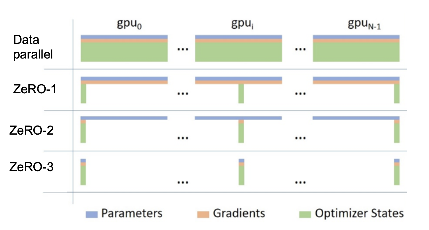
2.3 Storing Gradients and Parameters Without Redundancy (ZeRO stages 2 & 3)

We can take the partitioning idea further and do it for parameters and gradients as well as optimisation states.

In the forward pass:

ZeRO Stage 3 (Forward) — ZeRO Stage 3: forward pass

The first node broadcasts the parameters for the first section of the model.
All nodes complete the forward pass for their data for the first section of the model.
They then throw away the parameters for first section of the model.
Repeat for second section and so on to get the loss.

And the backward pass:

ZeRO Stage 3 (Backward) — Zero Stage 3: backward pass

The final node broadcasts its section gradients.
Each backpropagate their own loss to get the next gradients.
As before, final node accumulates and averages all gradients (reduce), calculates gradient update with optimiser and then broadcasts the results, which can be used for the next section.
Once used, all gradients are thrown away by nodes which are not responsible for that section.
Repeat for penultimate section and so on to complete the gradient updates.

If we have N cores, we now have an Nx memory footprint reduction from ZeRO.

A breather

That was the most complex part so feel free to check out these resources to make sure you understand what’s going on:

It’s all downhill from here!

Benefits of ZeRO

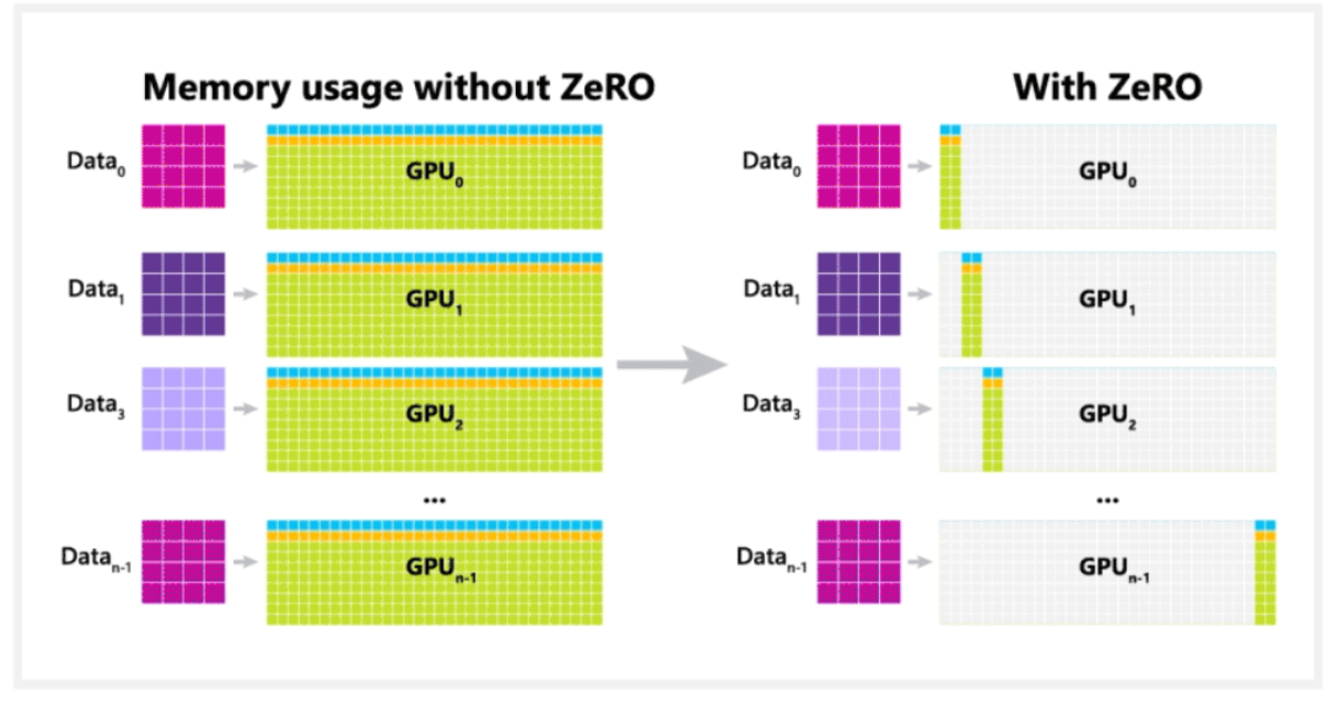
Overall, ZeRO removes the redundancy across data parallel process by partitioning optimizer states, gradients and parameters across nodes. Look at how much memory footprint we’ve saved!

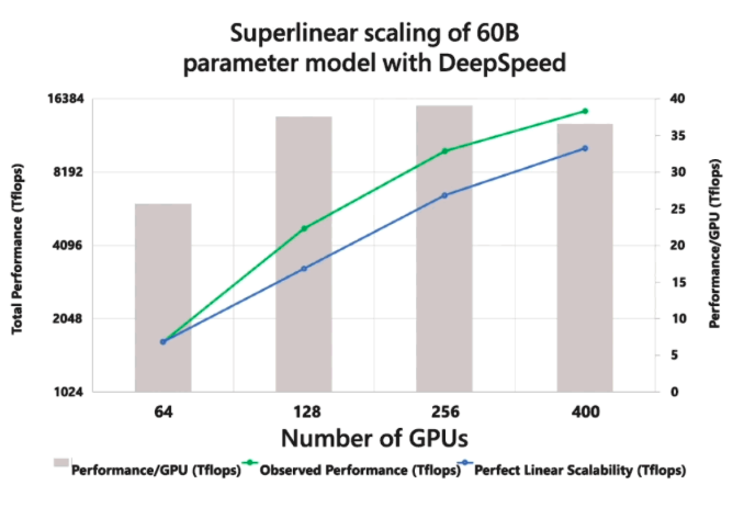
DeepSpeed Benefits — Benefits of DeepSpeed

One surprising thing about this approach is that it scales superlinearly. That is, when we double the number of GPUs that we’re using, we more than double the throughput of the system! In splitting up the model across more GPUs, we leave more space per node for activations which allows for higher batch sizes.

Superlinear Scale of DeepSpeed vs Perfect Scaling

2.4 Tensor Slicing

Most of the operations in a large ML model are matrix multiplications followed by non-linearities. Matrix multiplication can be thought of as dot products between pairs of matrix rows and columns. So we can compute independent dot products on different GPUs and then combine the results afterwards.

Another way to think about this is that if we want to parallelise matrix multiplication across GPUs, we can slice up huge tensors into smaller ones and then combine the results at the end.

For matrices \(X = \begin{bmatrix} X_1 & X_2 \end{bmatrix}\) and \(A = \begin{bmatrix} A_1 \\ A_2 \end{bmatrix}\), we note that:

\[XA = \begin{bmatrix} X_1 & X_2 \end{bmatrix} \begin{bmatrix} A_1 \\ A_2 \end{bmatrix}\]

For example:

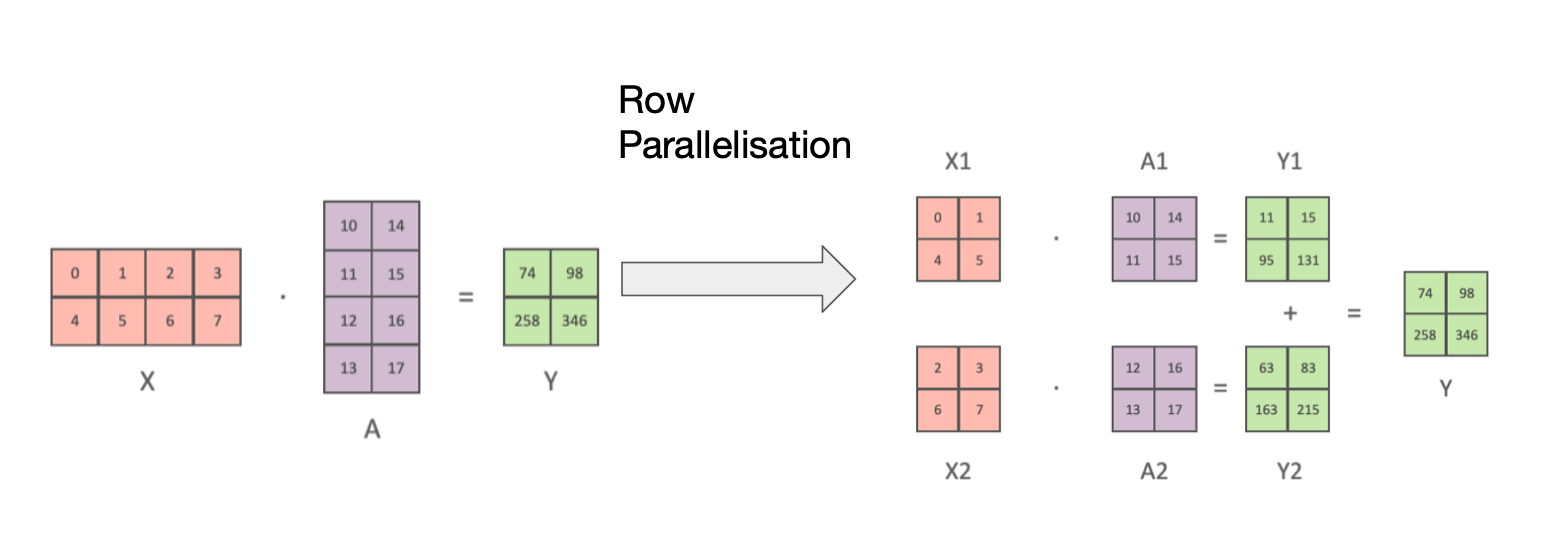
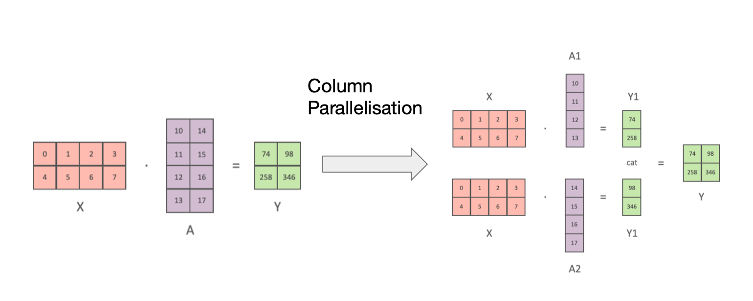
However if there is a non-linear map after the M e.g. if \(Y = \text{ReLU}(XA)\), this slicing isn’t going to work. \(\text{ReLU}(X_1A_1 + X_2A_2) \neq \text{ReLU}(X_1A_1) + \text{ReLU}(X_2A_2)\) in general by non-linearity. So we should instead split up X by columns and duplicate M across both nodes such that we have:

\[Y = [Y_1, Y_2] = [\text{ReLU}(X A_1), \text{ReLU}(X A_2)] = XA\]

For example:

Note: normally we think of A acting on X by left multiplication. In this case X is our data and A is the weights which we want to parallelise. Through taking transposes we can swap the order of the geometric interpretation so we can think of the above as linear map A acting on our data X and still retain the slicing.

2.5 Gradient Checkpointing

In our description of ZeRO each core cached (held in memory) the activations for it’s part of the model.

Regular backprop — The top layer represents the activations in the model populating during the forward pass and the lower layer, the gradients populated in the backward pass. The first circle is the input data and the bottom right is the loss.

Suppose we had extremely limited memory but were flush with compute. An alternative approach to storing all the activations would be to simply recompute them when we need in the backward pass. We can always recompute the activations by running the same input data through a forward pass.

Memory poor backprop — Here each activation is computed just before it's needed using forward passes.

This recomputing approach saves lots of memory but is quite compute wasteful, incurring m extra forward passes for an m-layer transformer.

A middle ground approach to trading off compute and memory is gradient checkpointing (sometimes known as activation checkpointing). Here we store some intermediate activations with \(\sqrt m\) of the memory for the cost of one forward pass.

2.6 Profiling etc

While not strictly causing any code optimisations, DeepSpeed provides developer friendly features like convenient profiling and monitoring to track latency and performance. We also have model checkpointing so you can recover a model from different points in training. Developer happiness matters almost as much as loss!

Check out the docs for more info!

3. In Pictures

Animated Video from Microsoft: warning, it’s a little slow.

4. In Code

The full DeepSpeed library, with all the hardware level optimisations, is open-sourced. See the core library, the docs and examples.

For an annotated and easier to follow implementation see Lab ML’s version.

5. Using DeepSpeed

DeepSpeed integrates with PyTorch and TensorFlow to optimize training.

In PyTorch we only need to change 4 lines of code to apply DeepSpeed such that our code is optimised for training on a single GPU machine, a single machine with multiple GPUs, or on multiple machines in a distributed fashion.

First we swap out:

model = model.to(device)
optimizer = torch.optim.Adam(model.parameters(), lr=1e-4)

with initialising DeepSpeed by writing:

ds_config = {
  "train_micro_batch_size_per_gpu": batch_size,
  "optimizer": {
      "type": "Adam",
      "params": {
          "lr": 1e-4
      }
  },
  "fp16": {
      "enabled": True
  },
  "zero_optimization": {
      "stage": 1,
      "offload_optimizer": {
         "device": "cpu"
      }
  }
}

model_engine, *_ = initialize(model=model_architecture,
                       model_parameters=params,
                       config = ds_config)

Then in our training loop we change out the original PyTorch…

for step, batch in enumerate(data_loader):
    # Calculate loss using model e.g.
    output = model(batch)
    loss = criterion(output, target)

    loss.backward()
    optimizer.step()

for:

for step, batch in enumerate(data_loader):
    # Forward propagation method to get loss
    loss = ...

    # Runs backpropagation
    model_engine.backward(loss)

    # Weights update
    model_engine.step()

That’s all it takes! In addition, DeepSpeed’s backend has also been integrated with HuggingFace via the Accelerate library.

That’s All Folks!

There’s a lot of clever improvements that go into the special sauce for training large models. And for users, with just a few simple code changes, DeepSpeed works its magic to unleash the power of all your hardware for fast, efficient model training.

Happy training!

DeepSpeed's Bag of Tricks for Speed & Scale